Gravitational Waves and the Detection Challenge

Gravitational waves (GWs) are ripples in spacetime produced by violent astrophysical events, such as colliding black holes, merging neutron stars, or exploding stars. First predicted by Einstein in 1916, they were directly detected for the first time in 2015 by LIGO (Laser Interferometer Gravitational-Wave Observatory), ushering in a new era of multi-messenger astronomy.

LIGO operates two detectors separated by ~3,000 km: one in Hanford, WA and one in Livingston, LA. Each detector uses a laser interferometer with 4-km arms to measure spacetime distortions smaller than one ten-thousandth the diameter of a proton. This extraordinary sensitivity makes LIGO equally sensitive to an enormous variety of noise sources: seismic vibrations, thermal fluctuations in the mirrors, quantum shot noise, and even distant traffic. As a result, genuine GW signals are buried in a sea of noise that can look strikingly similar. However, signals are strongly correlated between the two detectors, whereas noise is not; this makes it possible to detect GWs.

The central idea of this project is to frame detection as hypothesis testing: given two segments of data from both detectors, are they consistent with noise? Or do they contain a GW signal? If the distribution of noise was known, for example if it was a Gaussian, then this would be a simple p-value test. However, the noise in these detectors is a complicated, non-Gaussian distribution. Luckily, modern generative AI algorithms excel at solving this exact problem. I used a normalizing flow to learn the probability distribution of noise. A new segment is then flagged as a GW candidate if it is assigned low probability under the learned noise model, i.e., if it looks like an outlier relative to what noise typically looks like. A big advantage of this approach is that we don't need labeled gravitational wave detections to train this algorithm; it is completely unsupervised. All we need are samples from the noise distribution.

Data

This project used a publicly available LIGO challenge dataset consisting of three classes of signals, each represented as a pair of time series (one per detector) of length 200 samples (corresponding to ~50 ms):

• Background noise — 100,000 samples containing only detector noise, with no GW signal present.
• Binary Black Hole (BBH) mergers — 100,000 samples containing the characteristic chirp waveform produced as two black holes inspiral and merge.
• Sine-Gaussian Low Frequency (SGLF) signals — 100,000 samples containing a short-duration sinusoidal burst, representative of core-collapse supernovae or other compact sources.

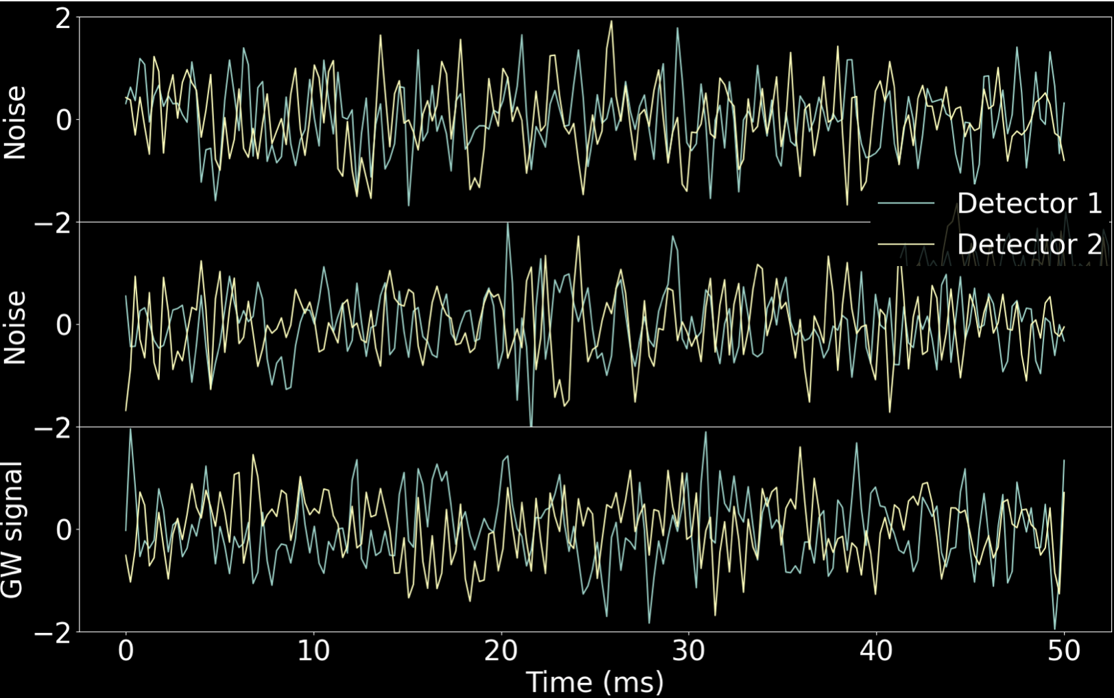
The raw data has shape (N, 2, 200) — \(N\) samples, 2 detectors, 200 time steps. The fundamental challenge is that noise and GW signals can look nearly identical in the time domain. The figure below shows three representative examples: the top two panels are pure noise, and the bottom panel is a BBH merger.

Feature Engineering: Cross-Spectral Density

Rather than training directly on the raw time series, I first transform each sample into a more informative representation: the cross-spectral density (CSD) between the two detectors.

The CSD between signals \(x(t)\) and \(y(t)\) (from detectors 1 and 2) is defined as: \[ C_{xy}(f) = X^*(f) \cdot Y(f), \] where \(X(f)\) and \(Y(f)\) are the discrete Fourier transforms of each detector's signal, and \(\ast\) denotes complex conjugation. Taking the absolute value \(|C_{xy}(f)|\) yields a 101-dimensional feature vector for each sample.

The CSD is a natural choice for GW detection for a key physical reason: a genuine GW signal arrives at both detectors (with a small time delay due to the finite speed of light), producing correlated power across frequencies. In contrast, noise at each detector arises from different local physical sources and is uncorrelated between detectors. The CSD therefore acts as a natural filter that is sensitive to coherent astrophysical signals while suppressing incoherent noise.

After computing the CSD, each sample is standardized with StandardScaler, and then compressed via Principal Component Analysis (PCA) retaining 70 components, which capture 95.08% of the total variance. This dimensionality reduction removes redundant features and makes the downstream modeling more tractable.

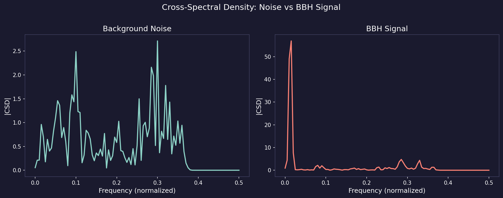
To make this concrete, the figure below shows the CSD for two representative samples. The noise sample (left) has cross-spectral power spread broadly and irregularly across frequencies with no dominant structure. The BBH sample (right) shows a sharp, dominant peak at low frequencies from the correlated chirp signal arriving at both detectors.

The Model: Normalizing Flows

A normalizing flow is a generative model that learns to transform a simple base distribution (here, a 70-dimensional standard normal) into an arbitrary complex distribution via a sequence of invertible, differentiable transformations. The key insight is the change-of-variables formula: given a bijective function \(f: \mathbb{R}^d \rightarrow \mathbb{R}^d\) that maps latent variables \(z\) to data \(x = f^{-1}(z)\), the log-probability of a data point is: \[\log p_X(x) = \log p_Z\big(f(x)\big) + \log \left| \det J_f(x) \right|,\] where \(p_Z\) is the base distribution and \(J_f\) is the Jacobian of \(f\). Because both \(f\) and its inverse are known analytically, we can evaluate exact log-likelihoods.

Architecture: Masked Autoregressive Flow

I used a Masked Autoregressive Flow (MAF), which constructs the bijection \(f\) autoregressively. For each dimension \(i\), the transformation is: \[ z_i = \frac{x_i - \mu_i(x_{1:i-1})}{\sigma_i(x_{1:i-1})}, \] where \(\mu_i\) and \(\sigma_i\) are neural network outputs that depend only on the preceding dimensions, enforcing the autoregressive structure via masking. This ensures the Jacobian is triangular and its determinant is simply \(\prod_i \sigma_i^{-1}\), making the log-likelihood tractable.

The flow consists of 3 such autoregressive layers, each preceded by a reverse permutation that shuffles the feature ordering so that different dimensions condition on each other across layers. Each \(\mu_i\) and \(\sigma_i\) network has a hidden layer of width 16 (not to be confused with the 70-dimensional input/latent space; this is simply the number of units inside the small networks that compute the per-dimension shift and scale). The model is trained with Adam (learning rate \(10^{-2}\), decayed to \(10^{-3}\) at epoch 30) on 80,000 background noise samples, minimizing the negative log-likelihood: \[ \mathcal{L} = -\frac{1}{N}\sum_{i=1}^N \log p_\theta(x_i). \]

Crucially, the flow is trained only on background noise — it has never seen a GW signal. The goal is simply to learn the noise distribution as accurately as possible.

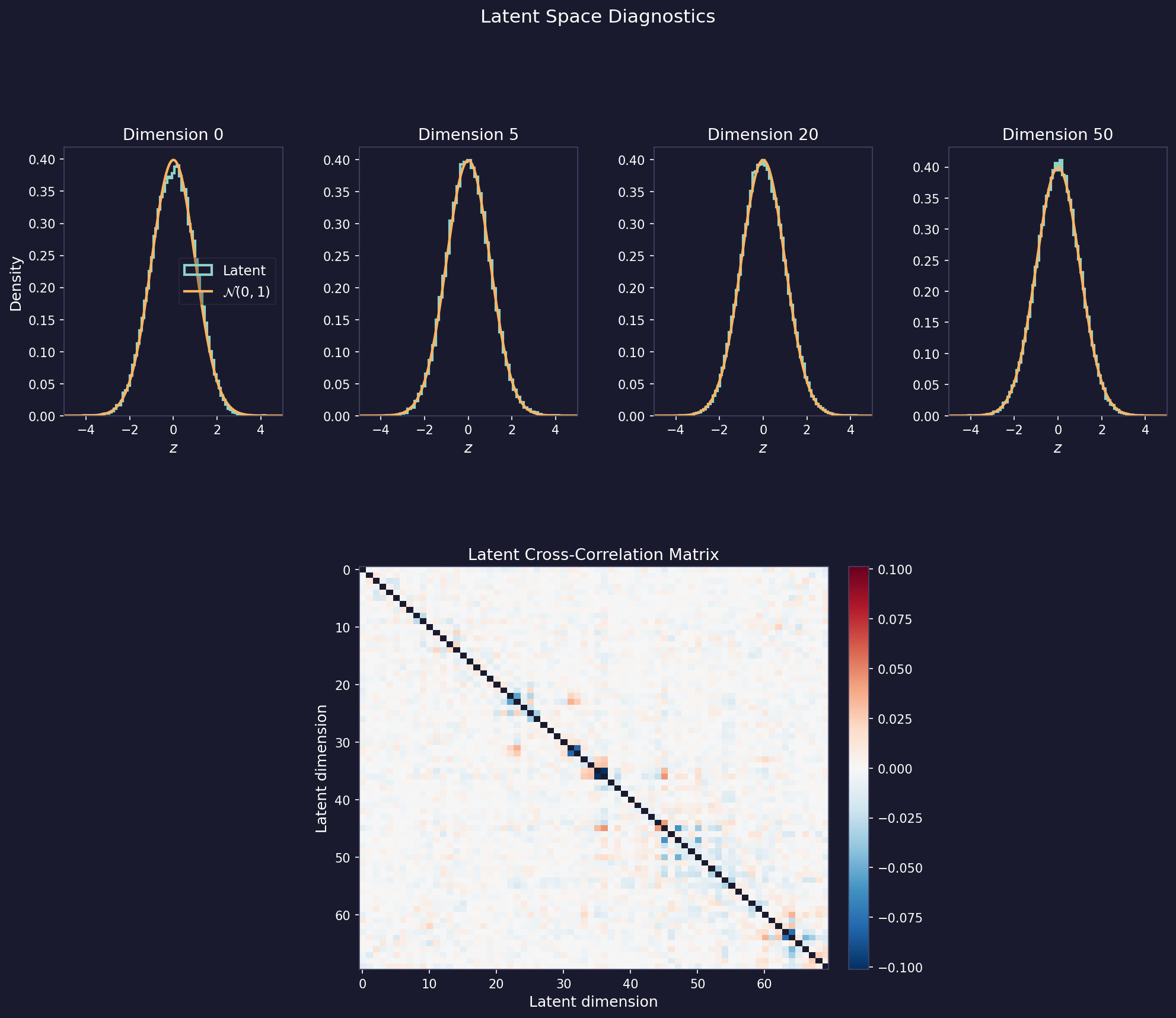
One way to check that the flow has converged is to verify that background noise samples, when passed through \(f\), produce latent coordinates \(z = f(x)\) that follow \(\mathcal{N}(0, I)\). If training succeeded, each coordinate \(z_i\) should be marginally distributed as a standard normal, and the coordinates should be mutually uncorrelated, since that is the base distribution the flow is trained to match. The figure below checks both: the histograms for four representative dimensions closely track the \(\mathcal{N}(0,1)\) curve, and the cross-correlation matrix of all 70 dimensions is near-diagonal, confirming convergence.

Detection as Anomaly Detection

Once the noise distribution is learned, GW detection becomes a simple thresholding problem. A new sample \(x\) is flagged as a GW candidate if \(\log p_\theta(x)\) falls below a threshold \(\tau\): \[ \hat{y}(x) = \begin{cases} \text{GW candidate} & \log p_\theta(x) < \tau \\ \text{noise} & \text{otherwise.} \end{cases} \] GW signals, having a different physical origin than detector noise, are expected to look like outliers under the learned noise model and receive anomalously low log-probabilities. By sweeping \(\tau\) across all values we trace out a Receiver Operating Characteristic (ROC) curve.

Results

The normalizing flow achieves an AUC (Area Under the ROC Curve) of 0.92 for SGLF signals and 0.89 for BBH signals, indicating strong discriminating power in both cases. The difference in performance is physically meaningful: SGLF signals are short sinusoidal bursts whose cross-spectral power is concentrated in a narrow frequency band, making them easy to identify as outliers. BBH chirps spread their energy across a broader range of frequencies and more closely resemble the noise distribution in cross-spectral space, resulting in a somewhat lower AUC.

This approach has a compelling advantage over purely supervised classifiers: the flow is trained exclusively on noise, requiring no labeled GW examples at training time. It can therefore generalize to new GW signals emitted from events for which we don't have good physical models.