Uncertainty Quantification

There are endless problems in physics where simple point estimates are not enough; we would prefer probability distribution functions (PDFs) of parameters. For example, cosmological and galaxy evolution studies can be sensitive to not only how far away a galaxy (or a group of galaxies) is, but to the probability that it is at a distance z. Beyond a measurement of the most likely parameter value, these PDFs also provide a sense of uncertainty via probabilities for all possible parameter values.

Every field, including astronomy, has a myriad of methods that provide different PDFs for the same parameter. These methods can be empirical (think data-driven, machine learning), or based on a physical model (and assumptions that come with it). Either way, which of the distributions are correct? How can we quantify the performance of these methods? In this blog, I will focus on the canonical astrophysics example of photometric redshift (photo-z) estimation. However, these methods are applicable in other contexts as well. You can think of redshift as a proxy for a galaxy's distance from Earth. Check out my blog on estimating distances to galaxies with deep learning for more on redshift!

Samples of Truth

The main difficulty stems from the fact that we do not know the true PDFs. For a galaxy, we estimate its distance (z) based on its images (x). Our algorithms therefore provide an estimate of the PDF conditioned on the galaxy images (x), or a conditional density estimate (CDE) \(\tilde{P}(z|x).\) If we know the true conditional density \(P(z|x)\), then we can use many metrics that measure "distances" between probability distributions, such as KL divergence, Earth mover's distance, or CDE Loss. The CDE loss is particularly useful because it can be estimated even when the true distribution is not known (more on this below). It is an extension of the mean squared error loss and is defined as: \[L_\mathrm{CDE}(P,\tilde{P}) = \int\int[P(z|x) - \tilde{P}(z|x)]^2dzdP(x).\] If \(P(z|x)\) is not available, then our only option is to use samples from it.

We can obtain a very accurate ("true") measurement of distance via spectroscopy, however that gives us only a single sample from \(P(z|x)\). Even if we make multiple spectroscopic measurements, that does not mean we will have multiple samples from \(P(z|x)\). We will only have multiple samples from \(P(z|s)\), where \(s\) is the spectrum of a galaxy; ¹ this does not help us with \(P(z|x)\). In short, since the true conditional density \(P(z|x)\) is not available, we will use many pairs of \((z,x)\) (test dataset), obtained via spectroscopic measurements, to evaluate the performance of these algorithms.

Methods

CDE Loss

As mentioned above, the CDE loss between the true and estimated distributions cannot be calculated if \(P(z|x)\) is not known. However, it can be estimated up to a constant with the following: \[\begin{align} L_\mathrm{CDE}(P,\tilde{P}) &= \int\int[P(z|x) - \tilde{P}(z|x)]^2dzdP(x) \\ &= \int\int [P^2(z|x) + \tilde{P}^2(z|x) - 2P(z|x)\tilde{P}(z|x)]dzdP(x) \\ &= \mathbb{E}_x\big[\int\tilde{P}^2(z|x)dz\big] - 2\mathbb{E}_{x,z}\big[\tilde{P}(z|x)\big] + K_P, \end{align}\] where \(\mathbb{E}\) represents averaging over samples in the test dataset. Because the constant \(K_P\) is unknown, this estimate is only useful for comparing the performance of multiple predictions \(\tilde{P}.\) Methods with lower \(L_\mathrm{CDE}\) are considered to be better. In fact, it can be used as a loss function.

PITs and P-P Plots

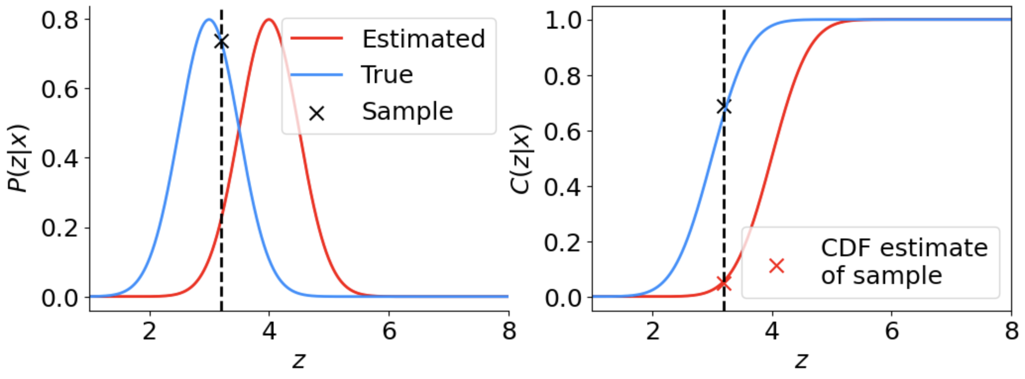
Suppose that the true conditional density is a Gaussian, \(P(z|x) = N(\mu_\mathrm{true},\sigma_\mathrm{true})\), and our predicted CDE is also a Gaussian with the same \(\sigma_\mathrm{true}\) but centered at a different location, \(\tilde{P}(z|x)=N(\mu_\mathrm{pred},\sigma_\mathrm{true})\). Figure 1 illustrates both distributions, along with a single sample point (\(z_i\) shown as an X) from our test dataset. The right panel shows the cumulative distribution functions (CDFs) of these PDFs. Notice how when we use the value \(z_i\) to calculate its estimated probability or CDF (with the red estimated CDE), we obtain values that are very different from truth.

Indeed, CDFs have a well-known property which we can exploit. Given a random variable \(Y\) with CDF \(C_{Y}\), the transformed variable \(\gamma=C_Y(Y)\) (also known as probability integral transforms, or PITs) will follow a uniform distribution. This can be shown with a few lines of math: \[\begin{align} C_\gamma(y) &= P(\gamma \le y) \\ &= P(C_Y(Y) \le y) \\ &= P(Y \le C_Y^{-1}(y)) \\ &= C_Y(C_Y^{-1}(y)) \\ &= y. \end{align}\] Therefore, since the CDF of \(\gamma\) is linear, \(\gamma\) follows a uniform distribution. This means that if we have a bunch of samples \(z_i\) from \(P(z|x)\), and we calculate \(\gamma_i=C_{z}(z_i|x)\), then \(\gamma\) will follow a uniform distribution. This is illustrated in the left panel of figure 2. Importantly, if we calculate \(\tilde{\gamma}_i=\tilde{C}_{z}(z_i|x)\) from our estimate \(\tilde{C}_{z}\), then \(\tilde{\gamma}_i\) will be uniform if and only if \(\tilde{C}_{z} = C_{z}\), i.e., if our estimated PDF is the true PDF. If this is not the case, then \(\tilde{\gamma}\) will not be uniform. This is illustrated in the right panel of figure 2.

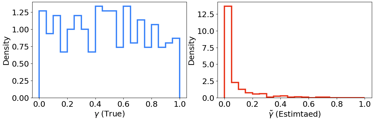
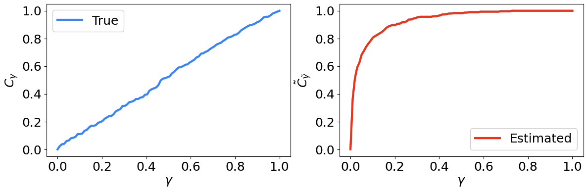
Figure 3 shows the CDFs of both \(\gamma\) and \(\tilde{\gamma}\). Indeed we see that the left panel shows a linear relationship, whereas the right panel shows a significant deviation from linearity. These figures are examples of P-P plots, because we are plotting the empirical CDF against our estimated one.

Intuitively, we are simply checking whether the CDE conforms to the frequentist interpretation of probability. Using test samples, we are checking whether the fraction of times samples fall within an arbitrary interval [\(z_1,z_2\)] is equal to the integral of the CDE between [\(z_1,z_2\)]. If the CDE is well-calibrated, then this should be true. We are checking for coverage probability.

As mentioned previously, we unfortunately will not have many samples from \(P(z|x)\). Instead, we will only have a single sample from each \(P(z|x_i)\), which are represented by the pairs \((z_i,x_i).\) As a result, we can only perform the above calculations globally — we can calculate \(\tilde{\gamma}_i\) for each object, and check if they are uniform. Similarly, we can estimate the CDE loss only globally. Ideally, we would also like to check conditional coverage. Across input space (\(x\)), the coverage probability can be incorrect in equal but opposite ways, making the global coverage look correct. That is a future blog post!