Measuring Distances to Galaxies with Next-generation Telescopes

The Nancy Grace Roman Space Telescope is a next-generation space-based observatory that will provide high-resolution images of hundreds of millions of distant and faint galaxies. Think Hubble Space Telescope (HST), but over an area roughly 10,000x the size of the moon! Estimating distances to these galaxies will be crucial for studies of galaxy evolution, cosmology, and supernovae.

Due to the expansion of space, light emitted by a distant galaxy gets stretched as it travels towards us. The amount of stretching — the redshift (z) — can be used as a proxy for distance. Reliably measuring a redshift involves a costly method called spectroscopy. It is especially difficult to measure the redshifts of distant, faint galaxies, which represent the majority of Roman observations. As a result, less than 1% of faint Roman galaxies will have reliable redshift measurements. For the remaining 99%, scientific analyses will heavily rely on redshift measurements from the images directly, called photometric redshifts (photo-z's).

This sounds like a machine learning (ML) problem: there is a complicated, non-linear relationship between galaxy images and their redshifts, and we can learn it with a training set (obtained via spectroscopic measurements of redshifts, or spec-z's). Indeed, Convolutional Neural Networks (CNNs) have been used previously for this exact purpose (see for example this paper). However, previous studies have been limited to nearby, bright galaxies with low-resolution ground-based imaging. In this work, our aim was to see if similar deep learning methods can be used on Roman-like datasets of faint, distant galaxies. In addition, we explored self-supervised methods and developed our own semi-supervised Photo-z Inference with a Triple-task Algorithm (PITA) that can learn from hundreds of millions of unlabeled data; PITA will be crucial for Roman's image-rich but label-scarce datasets.

Roman-like Data before Roman

To test deep learning algorithms, we required a Roman-like imaging dataset which also included redshift labels to train with. HST has similar resolution and wavelength coverage to Roman, making it a natural choice. We curated a catalog of ~100,000 HST images, ~20,000 of which have reliable redshift labels. Each galaxy has four images in four different filters: F606W, F814W, F125W, F160W. This data was collected as part of the CANDELS survey. While Roman will have 3 orders of magnitude more data (!), our HST dataset was sufficient for prototyping deep learning algorithms.

Interlude: Magnitudes and Colors in Astronomy

In astronomy, we measure brightness using the logarithmic magnitude system. It is an interesting topic, and I encourage you to read more about it. In short, if you add up all the light coming from a galaxy or a star in a certain wavelength window, and call it \(f\) (flux), the magnitude is defined as: \[m=-2.5\mathrm{log}\frac{f}{f_\mathrm{ref}}.\] \(f_\mathrm{ref}\) is some reference flux, and it varies between different magnitude systems. Traditionally, fluxes of specific reference stars (like Vega) have been used as \(f_\mathrm{ref}\). More recently, the AB magnitude is more commonly used.

Magnitude is measured per filter, so two filters \(i\) and \(j\) will have different magnitudes \(m_i\) and \(m_j\). For example, if a star is more red than blue, then it will have a lower magnitude in the red filter (remember the negative sign in the magnitude definition!). To quantify this, we define color as the difference in magnitudes \[c_{i,j}=m_i - m_j.\] Colors strongly correlate with many properties of galaxies, including redshift. Therefore, before deep CNNs allowed us to use the images directly, astronomers used colors and magnitudes to estimate redshifts.

Methods and Results: Surprising Lessons

With ~100,000 galaxy images and ~20,000 redshift labels, we were able to test three different machine learning strategies:

• Fully-supervised learning — This is the most common and well-known learning strategy, where only the labeled data are used to minimize a loss function that directly compares predicted labels to ground-truth values.
• Self-supervised learning — Unlike fully-supervised learning, self-supervised techniques create pseudo-labels from the data or rely on the training of surrogate tasks. Common examples include image reconstruction, predicting masked pixels, or creating different images of the same object and identifying them as a pair. The goal is to use unlabeled data to learn low-dimensional (latent) representations that are useful for downstream tasks such as classification or regression. Then, the labeled data can be used to fine-tune the network for a specific task, such as redshift prediction. In this work, we used self-supervised contrastive learning (explained below).
• Semi-supervised learning — This learning strategy can combine the best aspects of fully and self-supervised approaches, by simultaneously training with unlabeled and labeled data and minimizing a loss function that combines a self-supervised loss with a prediction loss. The PITA algorithm we developed is semi-supervised.

The fully-supervised algorithm is straightforward: we trained a ConvNeXt¹ CNN to predict redshift from images, using only the labeled data. We compared the deep learning algorithms to a traditional photometry-based multi-layer perceptron (MLP). Photometry is a technique that essentially involves adding up all the light of a galaxy in a single filter. The photometry-based MLP is trained to predict redshift from the total light in all four filters. This baseline represents how photo-z's were obtained before deep learning.

Table 1 shows results of the different methods using three evaluation metrics, based upon the normalized difference between the true (\(z_\mathrm{ref}\)) and predicted (\(z_\mathrm{pred}\)) redshift, \(\Delta{z} = \frac{z_{\text{ref}}-z_{\text{pred}}}{1+z_{\text{ref}}}\):

• The Bias \(\langle \Delta{z} \rangle\), defined as the mean of \(\Delta{z}\), which measures the average value of the prediction error.
• The normalized median absolute deviation (NMAD), defined as \(\sigma_{\text{NMAD}} = 1.4826\times\text{Median}\Big(|\Delta{z} - \text{Median}(\Delta{z})|\Big)\), which provides a robust estimate of the spread in prediction errors.
• The outlier fraction \(f_{\text{outlier}}\), defined as the fraction of objects with \(|\Delta{z}|>0.15\), which assesses the rate of catastrophic failures.

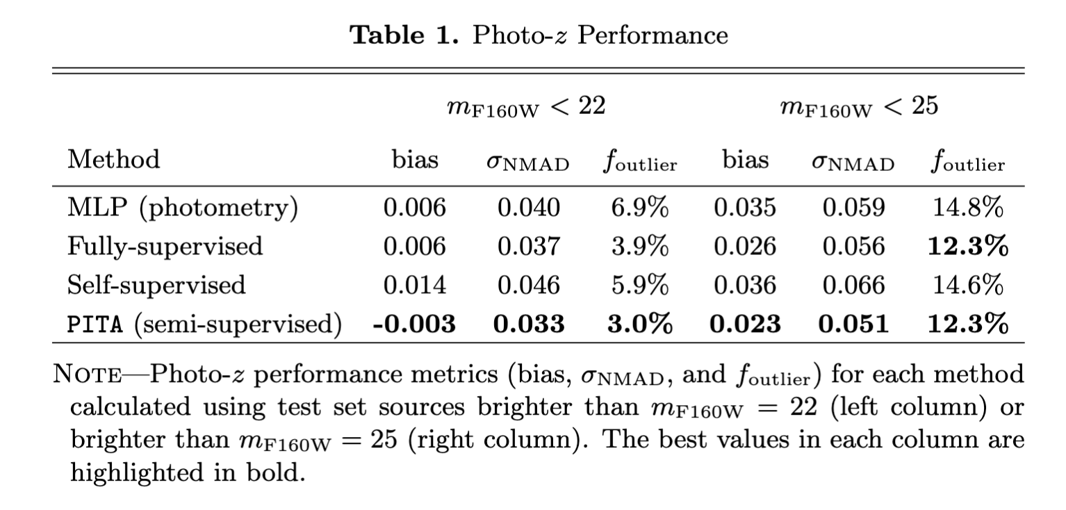
Our PITA algorithm performs best across the board, followed by the fully-supervised network. Surprisingly, the self-supervised + fine-tuned network does worse than the fully-supervised network. In order to understand this behavior, we must first understand how contrastive learning works.

Contrastive Learning

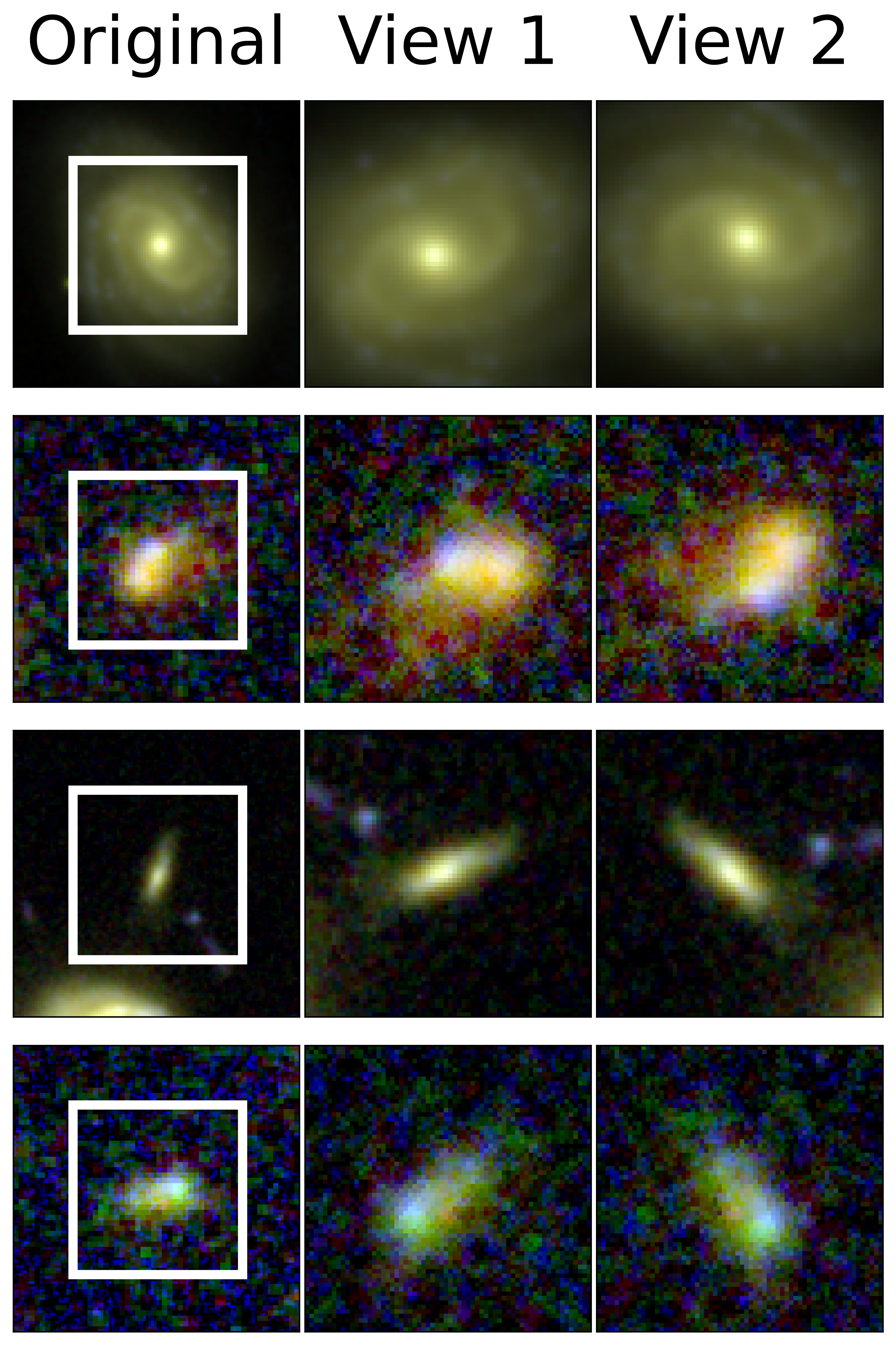
Contrastive learning offers a framework for constructing latent vectors (low-dimensional representations) of galaxy images that are invariant to specific transformations or views of the data. The goal is to learn representations that capture intrinsic features of galaxies while remaining robust to our chosen augmentations. For this work, we chose random horizontal flips, random rotation, jitter (randomly moving the center), and Gaussian noise.

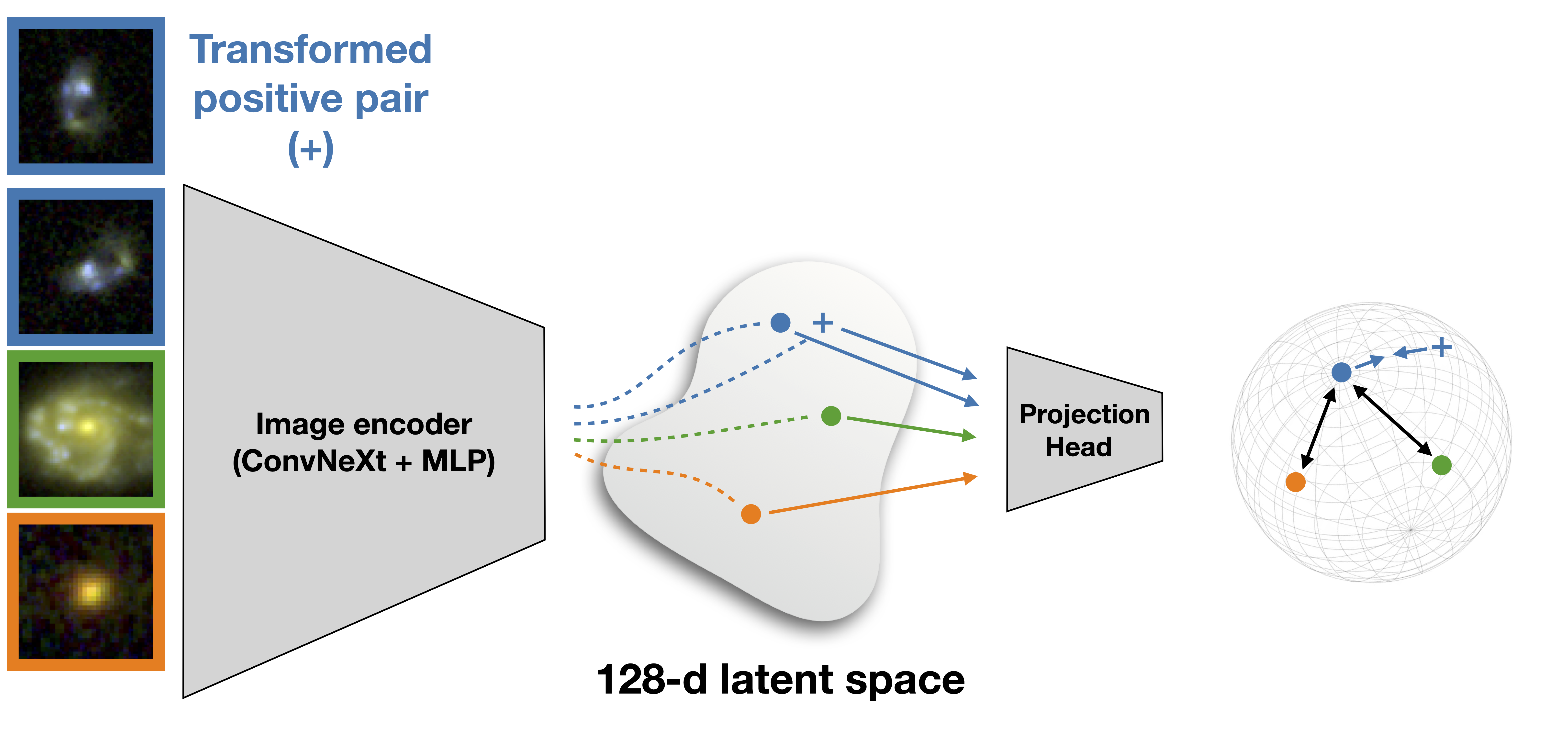
In practice, we implemented MoCo contrastive learning. We started by augmenting each image \(x\) using our chosen set of transformations (T) to generate new images \(x^t=T(x)\). Augmented images derived from the same initial image (\(x_i^t,x_{i^+}^t=T(x_i),T(x_i)\)) form a "positive pair" (see figure 2), while those originating from different initial images (\(x_i^t,x_j^t=T(x_i),T(x_j)\)) are labeled as "negative pairs". The training process then aims to maximize some measure of similarity between positive pairs in latent space. Typically, the cosine similarity (\(S_C\)), defined between two vectors \((\boldsymbol{A},\boldsymbol{B})\), is used: \[S_C(\boldsymbol{A},\boldsymbol{B}) = \frac{\boldsymbol{A}\cdot\boldsymbol{B}}{||\boldsymbol{A}||\;||\boldsymbol{B}||},\] where \(||\boldsymbol{A}||=\sum_{i}A_i^2\) is the magnitude of \(\boldsymbol{A}\). To prevent the trivial solution of collapsing all images to the same latent vector, the loss function incorporates an additional repulsive term that minimizes the similarity between negative pairs.

In MoCo, contrastive learning is framed as a dictionary look-up task. Given the latent vector \(\boldsymbol{q}\) of an image (obtained by passing the transformed image through the encoder), the latent vector \(\boldsymbol{k_+}\) of its positive pair, and the latent vectors \(\boldsymbol{k_i}\) of the remaining negative-pair images in the dictionary (\(K\) images), the InfoNCE loss function is defined as: \[l_{q} = -\text{log}\frac{\exp(S_C(\boldsymbol{q},\boldsymbol{k}_+)/\tau)} {\sum_{i=0}^{K}\exp(S_C(\boldsymbol{q},\boldsymbol{k}_i)/\tau)}.\] Here, \(\tau\) is a temperature hyperparameter, and the sum is performed over all the vectors in the dictionary, including the positive one \(\boldsymbol{k_+}\). This loss function can be interpreted as the categorical cross-entropy loss function for classifying \(\boldsymbol{q}\) as being the positive pair of \(\boldsymbol{k_+}\).

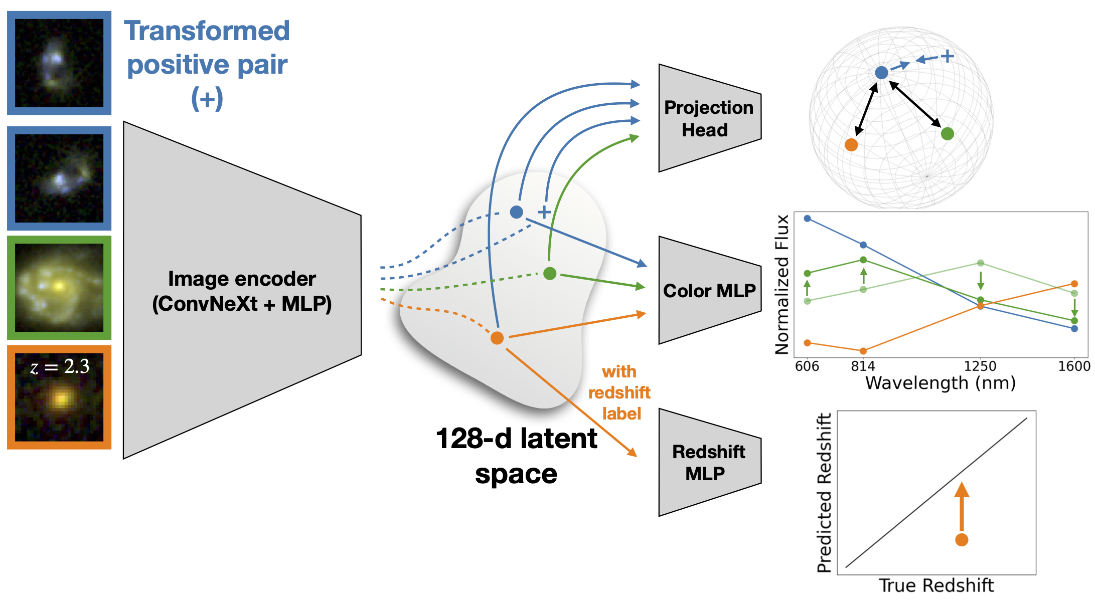
Figure 3 shows the architecture for the self-supervised algorithm. As the primary encoder, we used ConvNeXt. After training (see our paper for details), the 128-dimensional latent space offers an efficient representation of galaxy images.

Once the contrastive loss is minimized, we then used the labeled data to fine-tune the network for redshift prediction. In effect, this fine-tuning step is the same as training a fully-supervised algorithm with the encoder weights all initialized to the values learned from the contrastive pre-training. Table 1 shows the results post fine-tuning.

The success of this method rests on a key assumption: that the latent space efficiently encodes redshift information. We should not expect this a priori, since the loss function that is being minimized has no direct relation to redshift. In fact, the underperformance of this algorithm suggests that this assumption might not be true.

Looking at the Latents

The latent space compresses each galaxy image, which is 16,384-dimensional (64x64 pixels and 4 filters), into a 128-dimensional vector. In this sense, it offers a low-dimensional representation of galaxy images. However, 128 dimensions is still a lot, and impossible to visualize. To overcome this, we used the Uniform Manifold Approximation and Projection algorithm (UMAP) to visualize how the latent vectors correlate with physical properties. UMAP is a nonlinear dimensionality reduction algorithm that preserves both local and global topological structure. We applied it to project the 128-dimensional latent vectors into 2D UMAP embeddings, enabling us to assess how effectively they encode relevant information using scatter plots color-coded by the properties of interest.

Figure 4 shows results based on the 2D UMAP embeddings of the self-supervised algorithm's latent vectors. In the top panel, we divide the UMAP space into a grid and visualize the types of galaxies occupying each region by showing image cutouts of randomly selected samples. The middle panels show trends with \(m_\mathrm{F160W}\), F125W - F160W color, and reference or true redshifts (\(z_\mathrm{ref}\)). The bottom-left and middle panels show trends with full-width at half-maximum (FWHM; measure of size assuming the galaxy looks like a Gaussian), and specific star formation rate (sSFR; the rate of star formation divided by the mass of the galaxy). The bottom-right panel shows the predicted redshifts after fine-tuning (\(z_{pred}\)).

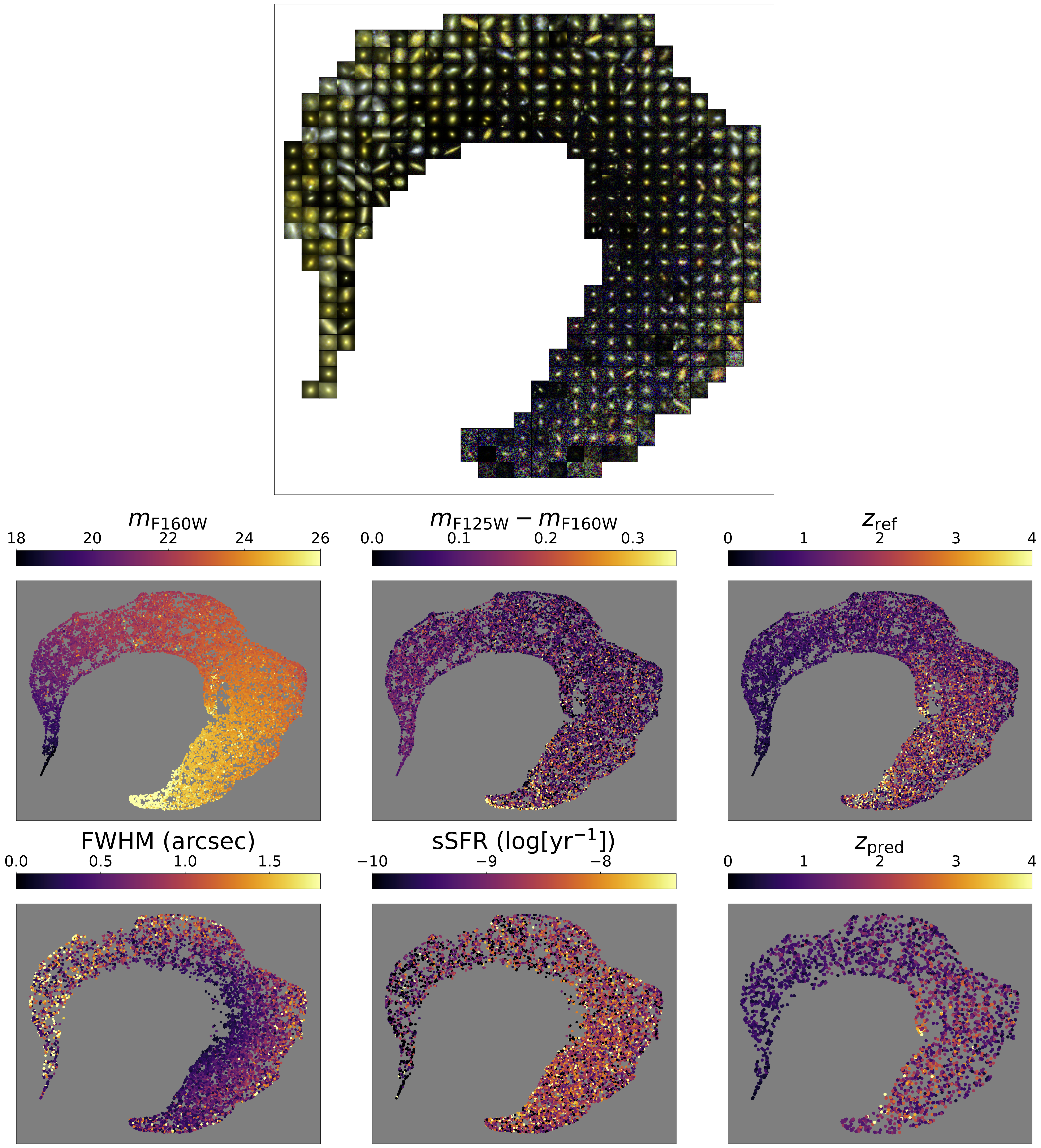
The top panel shows that the embeddings form a sequence of increasing magnitude (decreasing brightness) that runs clockwise around the arc, and a roughly orthogonal sequence of increasing size that extends radially outward. However, galaxies with different colors can be seen in neighboring cells, as can also be seen in the \(m_\mathrm{F125W}-m_\mathrm{F160W}\) color panel. As a result, sSFR and redshift, which are both strongly correlated with color, are likewise not well ordered.

These observed trends in the UMAP embeddings reflect the information encoded in the self-supervised latent vectors, and they are problematic. These vectors appear to primarily encode magnitude (brightness) and size, rather than color, redshift, or sSFR, leading to poor photo-z predictions. While these results were suprising at first, in hindsight they really aren't. The InfoNCE loss function defined above does not include any color or redshift terms, and separating galaxies by brightness and size seems to be enough to minimize this loss function. These are first-order properties that are easily obtained from the images. Color and redshift are higher-order properties that are more difficult to encode.

This qualitative UMAP analysis motivated us to develop PITA, which combines the contrastive loss with explicit objectives of predicting color and redshift, thereby guiding the latent space toward representations that are more informative for the downstream photo-z task.

PITA (Semi-supervised)

PITA jointly optimizes a contrastive loss \(L_\mathrm{contrastive}\), a color prediction loss \(L_\mathrm{color}\), and a redshift prediction loss \(L_z\), to yield a combined loss \(L_\mathrm{PITA}\): \[L_\mathrm{\texttt{PITA}} = L_{\text{contrastive}} + L_{\text{color}} + L_{\text{z}}.\] The contrastive loss is defined as the average of the InfoNCE loss (defined above), averaged over all images in the batch. For the redshift loss, we use the Huber loss function: \[L_z=L_\delta(y,f(\boldsymbol{x}))=\begin{cases} \frac{1}{2}(y-f(\boldsymbol{x}))^2, & \text{if $|y-f(\boldsymbol{x})|\leq\delta$},\\ \delta(|y-f(\boldsymbol{x})|-\frac{1}{2}\delta), & \text{if $|y-f(\boldsymbol{x})|>\delta$}, \end{cases}\] where \(y\) denotes the true redshift, and \(f(x)\) denotes the predicted redshift for input vector \(x\). We set the transition parameter to \(\delta=0.15\). For the color loss, we use an L2 loss function: \[L_{\text{color}} = \frac{1}{N}\sum_{i=1}^{N}|\boldsymbol{y}_i-\boldsymbol{f}(\boldsymbol{x}_i)|^2,\] where \(N\) is the batch size, \(\boldsymbol{y_i}\) is the true value, and \(\boldsymbol{f(x_i)}\) is the predicted value. Here, \(\boldsymbol{y_i}\) is a four-dimensional vector representing the three colors (F606W - F814W, F814W - F125W, and F125W - F160W) and a single magnitude (\(m_\mathrm{F160W}\)).

The contrastive loss does not require any labels to evaluate. Similarly, colors can be calculated from all the galaxy images, so all the data within a batch contribute to these two loss terms. In contrast, only labeled images contribute to the redshift loss. If a batch contains no labeled examples, the redshift loss is set to zero.

Figure 5 illustrates the architecture used for PITA. Similar to the previous architectures, the encoder consists of a ConvNext CNN followed by an \(\text{MLP}_\text{encoder}\), which together process the four-band input images and output 128-dimensional latent vectors. From this shared latent space, three task-specific MLPs further project these representations to calculate the loss:

• The projection head, which is a single-hidden-layer MLP with 128 neurons that maps the 128-dimensional latent vector to a 64-dimensional space in which the contrastive loss is computed.
• The color MLP (\(\text{MLP}_\text{color}\)), which consists of six hidden layers with [128, 128, 128, 128, 128, 64] neurons and outputs a 4-dimensional vector corresponding to F606W - F814W, F814W - F125W, F125W - F160W, and \(m_\text{F160W}\).
• The redshift MLP (\(\text{MLP}_\text{redshift}\)), which also consists of six hidden layers with [128, 128, 128, 128, 128, 64] neurons and outputs a scalar redshift.

Looking at PITA Latents

Figure 6 shows the 2D UMAP embeddings of the PITA latent vectors. In the top panel, galaxies that are near each other in embedding space exhibit similar morphologies, colors, and brightnesses. This is reflected in the smaller panels, which exhibit clear and smooth trends in magnitude, color, size (FWHM), sSFR, and redshift.

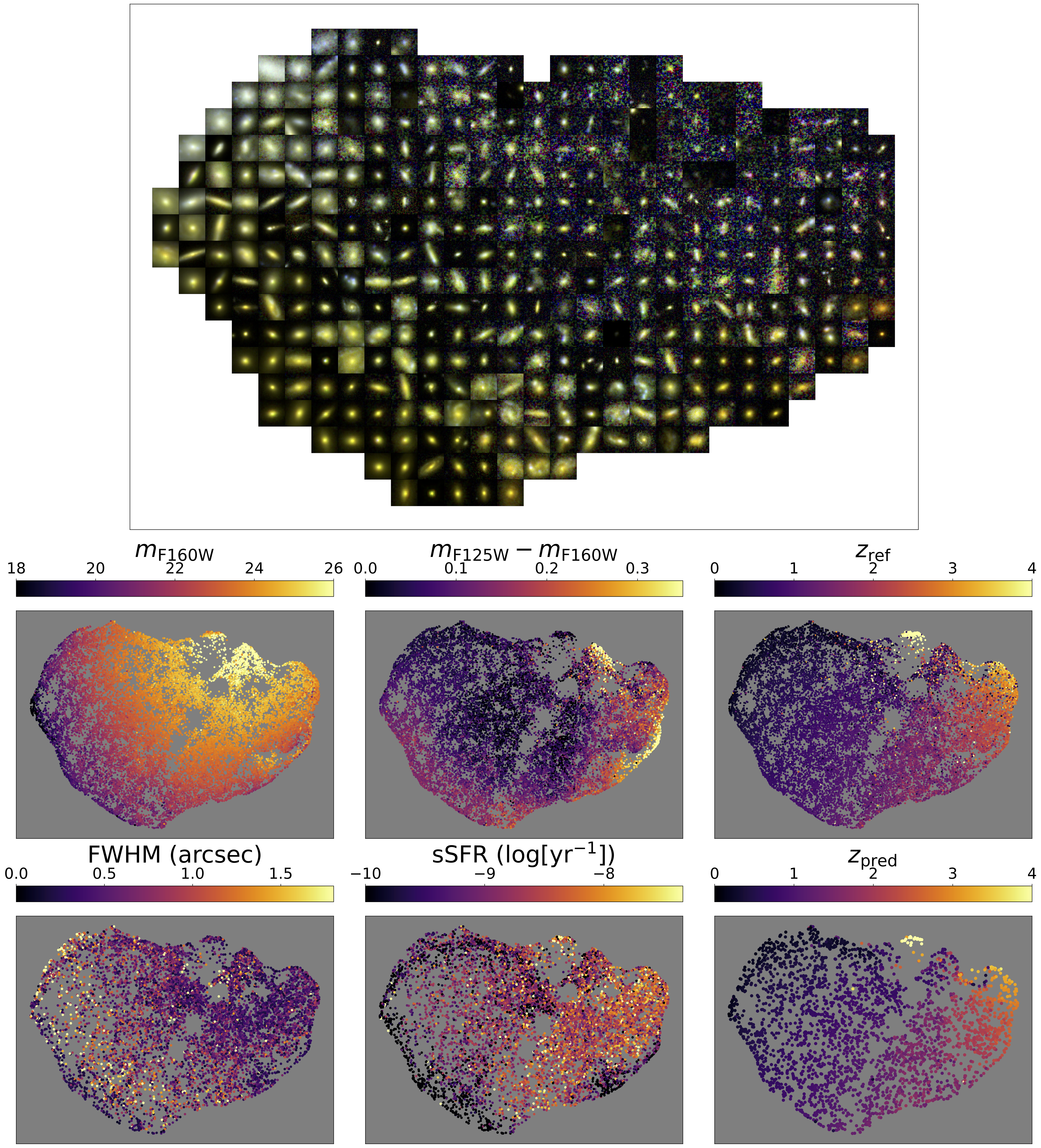
The smooth gradients of color, sSFR, and redshift across embedding space indicate that the color and redshift losses are properly aligning the PITA latent vectors to encode important galaxy properties. The fact that there is still a clear trend with size (FWHM) indicates that, while the redshift and color losses help to align the latent space, the contrastive loss still encourages the latent vectors to encode morphological information.

Scaling with the Number of Training Data

Deep learning can be viewed as a combination of feature extraction and regression. Initial layers learn to extract appropriate features from images, while final layers perform a simple regression from those features to estimate redshift. From this perspective, semi-supervised learning has a clear advantage over fully-supervised: the larger unlabeled data are used to learn informative features, and the much smaller set of redshift labels are used to train the regression.

Figure 7 compares the performance of PITA to the remaining ML methods as a function of the size of the redshift training set. Across all approaches, performance improved as the size of the labeled training set was increased, consistent with expectations for ML models. There appears to be an inflection point around ~10,000 data points, where the fully-supervised deep learning algorithm starts to outperform the photometry-MLP. This is not surprising; deep learning CNNs are data-hungry, but they can outperform classical ML in many applications when provided sufficient training data.

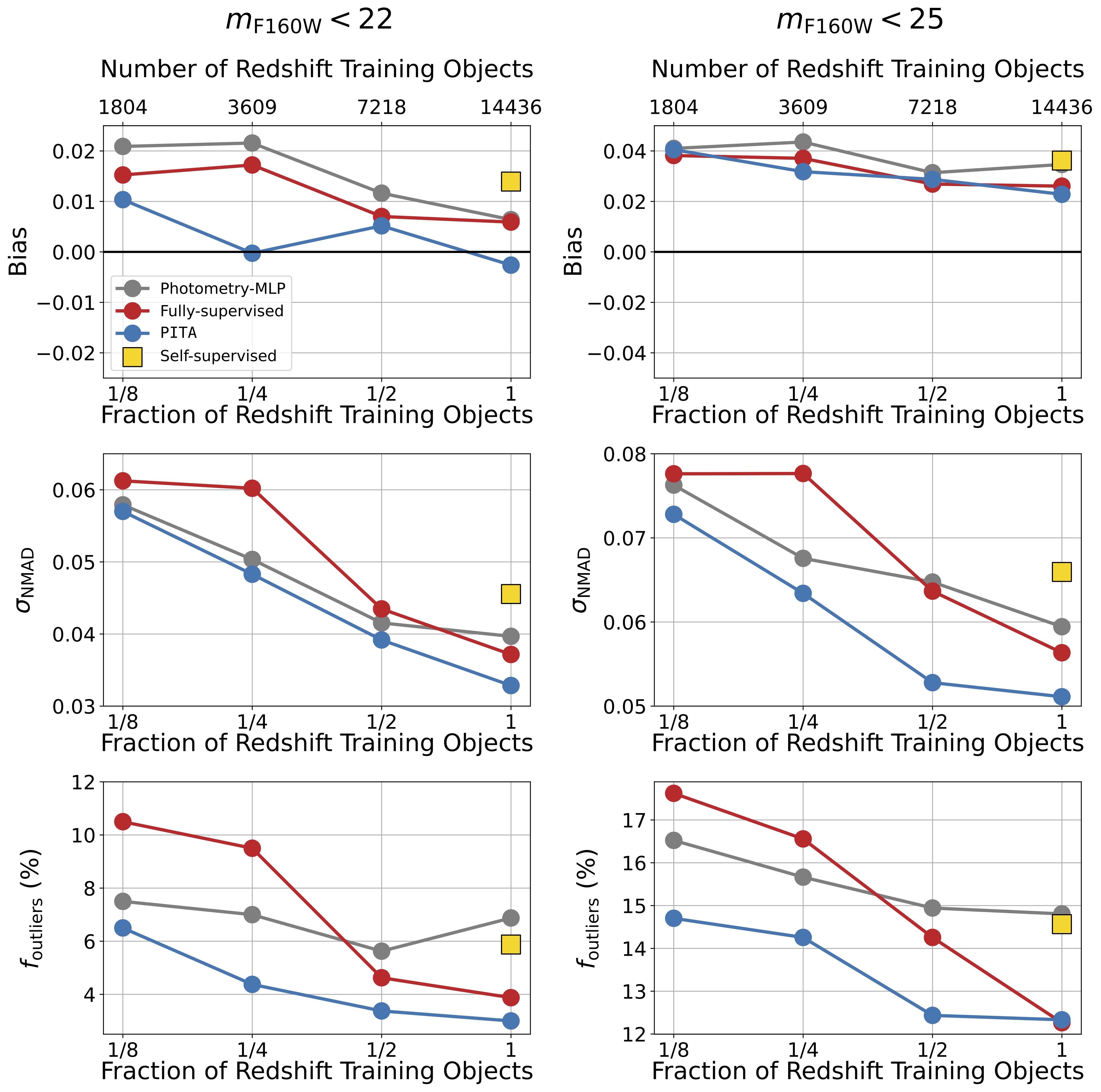
However, PITA outperformed all other methods across all performance metrics, even when very few redshift labels were used. This is because the contrastive and color losses take advantage of unlabeled data to learn informative latent vectors, and the small subset of labeled examples is then used to better align those vectors with a redshift loss. The PITA latent space is therefore well suited for interpolation between sparse training redshifts, allowing optimal use of samples that are limited in size.

As telescopes like Roman push toward higher-redshift samples and fainter galaxies, obtaining spectroscopic redshift labels will become increasingly difficult. The regimes of low and high number of available training objects (the ends of the x-axis in Figure 7) will correspond to faint and bright galaxies, respectively. Leveraging unlabeled objects will therefore become crucial for Roman. Methods like PITA that can effectively leverage the vast amounts of unlabeled data and that can exploit domain knowledge will yield the best possible photo-z estimates, helping to advance studies focused on cosmology, galaxy evolution, and transient science.